Even in 2016, cloud storage suffers from a significant problem - I/O latency. The scarce resource in the cloud may not be throughput but consistently low I/O latency. For example, see this link about AWS top 5 problems.

By Karl Cronburg and Ben England

End-user Perspective: Percentiles

Here we discuss the latency problem from a user perspective. If you are the user boiling mad from waiting 20 seconds for your directory to browse, you do not care what the average latency is - you only care what YOUR latency is RIGHT NOW. While impractical to guarantee good latency for every single I/O request, we certainly wish to guarantee that a large percentage of I/O requests are serviced within a reasonable amount of time. This is often reflected in

Service Level Agreements

(SLAs), defining a required level of performance to be delivered by the service provider to the user. For example, a distributed filesystem site may be asked to guarantee that in 95% of all cases a directory can be browsed in under 1 second, and 99% of all directory browsing operations complete in under 5 seconds. Or a block device service using RBD may be asked to guarantee that transactions for a database complete within 2 seconds 99% of the time. In statistical terms, this translates to the 95th percentile of directory browsing response times being no more than 1 second. Conclusion: Ultimately percentiles are far more relevant in the latency domain than averages, and percentiles as a function of time (i.e. for intervals under 1 minute), not percentiles over long time intervals (i.e. for hours).

Latency Measurement

There are two questions of interest to system administrators:

How do we measure system-level latency percentiles?
How do we measure changes in them over time?

However, tools are not typically setup to measure system-wide latency percentiles. With averages one can:

Take a per-thread average
Average of these averages weighted by number of IOPS gives system-level.

This however does not work for percentiles. For example, the fio benchmark reports per-thread percentiles and will even aggregate within a single host to get host-level latency. But in a distributed system there is currently no way to get fio to report cluster-level 95th percentile latency.

t.fio: (g=0): rw=randwrite, bs=1M-1M/1M-1M/1M-1M, ioengine=sync, iodepth=1
fio-2.1.10
Starting 1 process
t.fio: (groupid=0, jobs=1): err= 0: pid=18737: Fri Jan 9 20:27:08 2015
 write: io=20480KB, bw=1019.4KB/s, iops=0, runt= 20091msec
...
clat percentiles (msec):
| 1.00th=[ 1004], 5.00th=[ 1004], 10.00th=[ 1004], 20.00th=[ 1004],
| 30.00th=[ 1004], 40.00th=[ 1004], 50.00th=[ 1004], 60.00th=[ 1004],
| 70.00th=[ 1004], 80.00th=[ 1004], 90.00th=[ 1004], 95.00th=[ 1004],
| 99.00th=[ 1004], 99.50th=[ 1004], 99.90th=[ 1004], 99.95th=[ 1004],
| 99.99th=[ 1004]
...

Here we have per-thread percentiles but not cluster-level percentiles. fio does generate latency logs which are CSV-format tables of (time, response-time, direction, transfer-size) records. A typical distributed storage system could generate on the order of millions or even tens of millions of such records for IOPS-intensive workloads. There is ongoing work on the tools/fiologparser.py tool to enable it to produce percentile statistics showing variation in percentiles over time. Statistically it is difficult to infer system-level percentiles from component percentiles. Why is that? It is trivial to infer system-wide percentiles from per-thread results if all threads have same response time distribution (single-thread test is special case). But of course this is improbable in a large distributed storage environment. There are some statistical methods for estimation but they are highly complex and not typically embedded in commonly available libraries. As for time-varying latency, we need this feature to understand “when did the problem start and end?”, which is critical for performance monitoring and troubleshooting. For example, here’s what it might look like to have such statistics over time. This graph shows the difference between average latency (in red) and 99% latency (in light blue), and gives you an idea of the spread of the latency distribution and how that varies. For example, the maximum latency could be an outlier that never repeats, so it is not a reliable way to look at latency. However, maximum latency can determine whether I/O timeouts, etc. are experienced by a virtualized application.

Looking at just 95% latency for an entire Ceph Hammer (untuned) cluster during a simulated disk failure and recovery, using latency logs from 128 RBD devices, we get a graph like this (note: this problem is old news and upstream Ceph should address it).

This graph was not instantaneous to generate because we had to merge and process 30 million latency samples to do it, and this took about 30 seconds. On a larger cluster this would be much more expensive. However, if we processed 10-second intervals as they became available it would be a much more bounded problem. An optimized (using numpy and capable of streaming in the data as it becomes available) version of fiologparser produces the following graph in about the same amount of time with 1 second interval granularity (thus the extra spikes in latency seen):

Here’s the same dataset looking at 95% latency by each thread (y-axis is in microseconds instead of seconds x-axis uses 60-second time intervals). Note that per-thread latencies are very close, because there is no relationship between fio threads and an individual OSD - Ceph is designed to spread block device I/O requests across a large number of OSDs. Consequently a failure of one OSD affects all threads equally. If we were observing a flaky network interface at a client host, we would have seen a very different picture, with all threads on that host suffering high latency equally. So this graph can help us to infer where the source of the latency might be.

In summary, there are two benchmarks that will generate the raw data for cluster-level percentile-over-time calculations:

fio - with --write_lat_log option
smallfile - with --response-time Y option

Real-time system-wide latency measurement

A final step in this process would be to find a way to do this in real time, so that a system administrator could monitor latency throughout her portion of the cloud, get alerts when latency is exceeding SLA thresholds, and take action to correct problems before users even noticed them. This could be done in 1 of two ways:

Collect raw latency samples from individual threads throughout the cluster for a time interval of interest, merge and process them - this could be expensive, though compression could help reduce network overhead.
Do statistical reduction of samples right within the host or even the thread that generated them, so that we only have to merge the statistics from the samples, rather than the entire collection of samples.

First attempt - weighted average of per-thread percentiles
Second attempt - use histogram to represent latency samples

Weighted average of per-thread percentiles

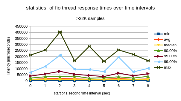
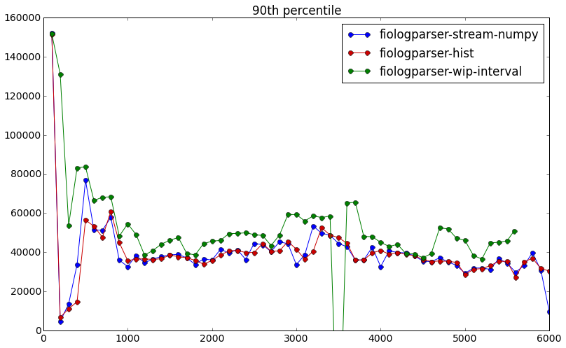
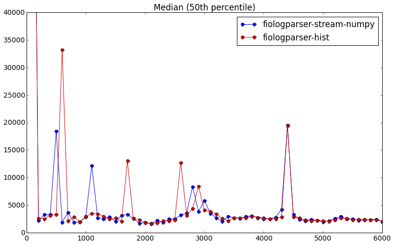
Although there is no way to precisely calculate percentiles of an entire system from per-thread percentiles, we at first try to estimate them. Comparison shown below using an iop weighted average estimation method with 4 ceph nodes and around 50 iops per node per bin (1000ms bins), as compared to merging latency logs across nodes and binning into windows according to end time: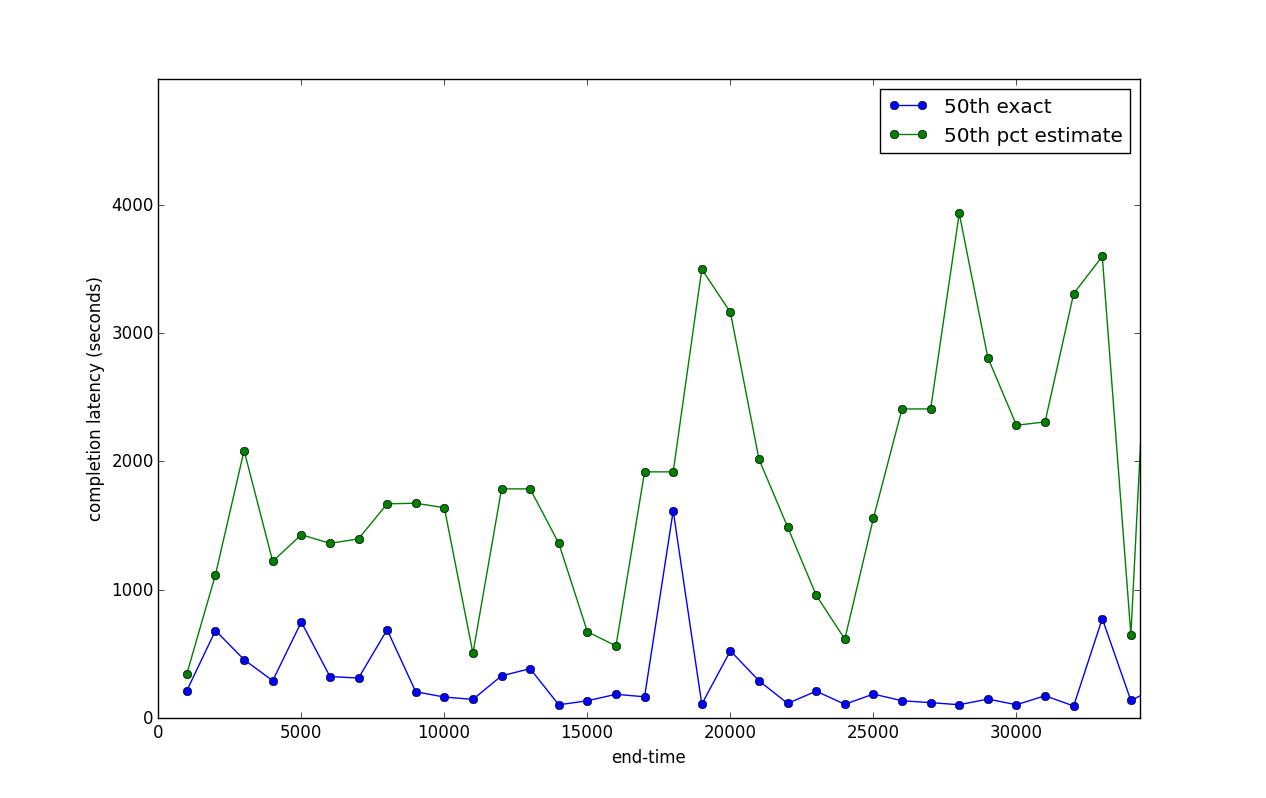

The estimation method, in this instance, appears to consistently overestimate the 50th percentile completion latency. This is likely due to small sample sizes with skewed distributions and outliers pulling the averaging of the estimation method way up. Similar and in some cases worse estimates are seen for 90th, 95th, and 99th percentiles - the higher the percentile, the more noise we see in estimations.

Methods used:

IOP weighted average estimation method:

where n is the number of iops for node i, and p is the 50th percentile calculated for the node using numpy.percentile.

Exact:

Merge all log files across nodes, bin operations into time windows, and use numpy.percentile to compute the 50th percentile of each time window.

Latency histogram method

In this method, we have each thread add incoming samples to a histogram for some fixed measurement interval, then output the histogram. We can treat the normalized histogram as an approximation of the probability distribution function (PDF), and can integrate the PDF to get a cumulative distribution function (CDF) - percentiles are then estimated from the inverse of the CDF.

Input:

clat / lat log file name, number of (logarithmically-spaced) bins to use per interval, initial bounds on the latency values to compute initial bins, and an interval width.

Algorithm:

Each interval gets a histogram.
Histogram bins computed in logarithmic-space with np.logspace
Histogram bounds given as power of 2, e.g. (0,30) to indicate a histogram with range [2^0, 2^30] .
Bins added dynamically as needed for each interval.
Histogram bins are incremented by the fraction of a request falling within the interval, meaning we get out weighted percentiles from computing the inverse of the CDF.
CDF computed with np.cumsum of the histogram, normalized by number of samples.
Percentiles are calculated by interpolating the inverse of the CDF, e.g. with np.interp (linear interpolation).

Current implementation on github.

Output:

Per-thread histogram for each interval for subsequent merging and system-wide percentile calculations. The strength of this method is that it is easy to merge per-thread histograms to obtain histograms for other aggregations, such as per-client histograms or cluster-wide histograms. This in turn gives us an inexpensive way to estimate percentiles that will work at large scale and with high-IOPS storage hardware such as NVDIMMs. The user can tradeoff space for accuracy by increasing the number of bins used. Logarithmically-spaced bins are used to more accurately reflect the skewed nature of distribution of latencies, and thus maintain fewer bins for each histogram. Logarithmic histogramming shown below for an interval with 40 bins.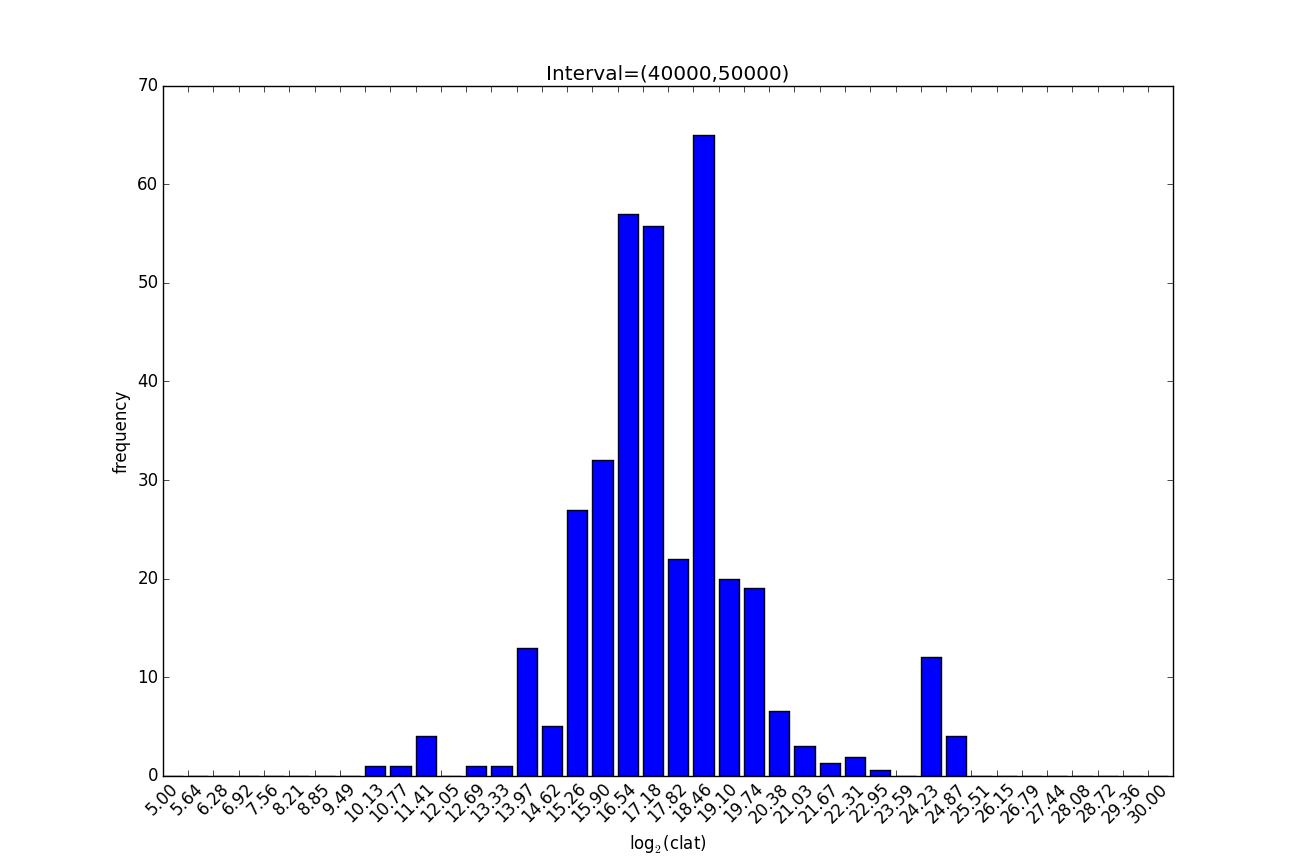

Accuracy:

Number of bins / bin width and number of samples impact accuracy. Accuracy is logarithmically bounded, i.e. the width of the bin in which a percentile falls can be viewed as the error in that percentile. What this means practically is that higher latency percentiles will be calculated less accurately than smaller latencies. In current test cases, this inaccuracy is easily mitigated by increasing the number of bins (extremely cheap to do, since each bin requires a mere 4 bytes). In contrast the real limiting factor in accuracy for our application appears to be sample size - we must choose an interval length of at least 10 seconds to get enough samples for 10% accuracy in the 95th percentile (similar for 90th and 99th). This interval will need to be tuned by the user - for instance we can get away with a much smaller interval on NVDIMMs.

Possible extension:

Auto-tuning the interval length in order to obtain a particular accuracy - i.e. we show the histogram building up to the user as samples come in, and then when enough samples are present we flush the histogram and plot data points for the desired percentiles.

Scalability:

Histograms are small data structures which can be kept in memory on the host being benchmarked. The main hurdle to overcome with scalability in calculating system-wide percentiles is the need to retain the histogram for all intervals in the event that a long-running IOP gets reported. In practice this occurs either when:

Something interesting is happening (disk failure, flaky NIC, …), or
Random noise / event in the system

The former is what we’re most interested in detecting, so we need some way to account for these long-running IOPs. In post-processing , this means first sorting the samples by request start time (n lg n) and doing a linear scan of the samples to figure out what intervals they belong to (n). In a live analysis outside benchmarking tool (fio, smallfile, ... .), the only reasonable solution is to have a log of when requests are first made so that we know when all samples in an interval have been accounted for, otherwise scalability is out the window (linear memory usage growth with time). In a live analysis with substantial changes to benchmarking tool , we can achieve scalability (constant memory usage) by building our weighted histograms in the benchmarking tool.

Fio Histograms:

Fio appears to use a similar histogramming method as above, as seen in the json output files. We leverage these existing histograms by outputting them every so often (in lieu of outputting every single IOP) and merging them on a centralized server for subsequently computing statistics / percentiles on.

Fio Histogram Output Format & Semantics:

When using CBT, each thread on each of the client hosts generates a file using a similar naming convention to the files fio already produces e.g. output.0_clat_hist.2.log.gprfc073 for the latency histograms generated on host gprfc073 in thread #2. Each row contains a comma-separated list of the bin frequencies, with the first column corresponding to milliseconds since the thread started running, the second column being the r/w direction (read=0, write=1), the third column being the block size, and the remaining 1,216 columns of frequency bins. Thus we have 1,219 columns total. Bin indices fall in the inclusive range [0,1215] and can be converted to millisecond bin latency values using the function plat_idx_to_val from stat.c in fio. A python implementation of this function can be found alongside our NumPy implementation of fiologparser . Implementation of histogram merging (across threads / hosts) and subsequent percentile calculations also available, with statistics reported in the same format as fiologparser.

Using fio with histogram output:

Checkout branch histograms of cronburg’s fio fork: cronburg@github:fio/tree/histograms
Build fio (make).
Point CBT at this version of fio. Running CBT will collect all the necessary *_clat_hist* files generated on each client.
On a fresh docker image of Fedora 23, the following packages are required / commands are run before running fiologparser:

dnf update &&
dnf install -y git python numpy python2-pandas Cython gcc redhat-rpm-config
git clone https://github.com/cronburg/fio.git && cd fio/tools
git fetch && git checkout histograms
curl -L -O http://cronburg.com/fio/z_clat_hist.1.log # Example log file
./fiologparser_hist.py z_clat_hist.1.log

At present this installs: python-pandas-0.17.1, numpy-1.9.2, Cython-0.23.4
Run NumPy version of fiologparser on *_clat_hist* files generated, e.g.:

$ /path/to/fio/tools/fiologparser_hist.py /path/to/logs/*_clat_hist*

Histogram Merging Algorithm:

Input: List of file(name)s containing histogram logs from fio
For each time interval (e.g. 100 milliseconds):

Read in the histograms corresponding to that interval, and merge all the histograms into a single system-wide histogram by taking the sum of each bin across hosts / threads.

For each system-wide histogram interval:

For each bin in the histogram:

If the latency value of the bin is less than or equal to the interval-length, leave the frequency value alone (all samples falling in that bin are given a weight of 100% because they fell completely in this time interval).
Else if the latency value of the bin is greater than our interval-length:

Weight the samples in the bin by the fraction of the bin value (latency value of the samples) by the fraction of the sample(s) falling in the interval.
Look at future intervals of the system-wide histogram, computing the fraction of the same bin’s effect of the future histogram on the current system-wide histogram. For example (interval = 100 ms) a bin value of 150 milliseconds with a single sample will have a weight of (150 - 100) / 150 = 0.5 on the 150ms bin of the system-wide histogram immediately before it.

Now weighted percentiles can calculated from each of the system-wide histogram by computing the cumulative sum and calculating the value at which the weighted frequencies add up to XX% of the total sum of the weighted frequencies. Linear interpolation ( np.interp ) is used to gain better accuracy.
Output: A stream of weighted percentiles, one for each interval.

Accuracy: We are able to calculate percentiles from histograms with excellent accuracy compared to calculating them from logs of every single IOP. Below are plots of the 99th, 95th, 90th, and 50th percentiles for a short run of fio with both *_clat_hist* (histograms - red line below) and *_clat.* (every single IOP - blue and green lines below). The blue and red lines use the exact same weighted-percentiles calculation, and so are directly comparable for accuracy. The green line is with the existing calculations in Mark’s wip-interval branch version of fiologparser.

With the speed and accuracy afforded to us by histogram output from fio, we can easily calculate finer-grained percentiles e.g. every one percent from the 50th to 99th percentile, and display this data to the user with e.g. a sliding bar on the side of the plot to change which percentile the graph is showing, or plotting the 3d surface with end-time and percentile (50 to 99) on the x and y axes, and percentile-value on the z-axis. Bumps in this surface “hiding” just above or below the slices we currently take (at 50, 90, 95, and 99) will become more readily apparent by visualizing the surface. Full IPython notebook comparing histogram method with logging every single IOP (plots above taken from here): https://www.cronburg.com/fio/Histogram-Accuracy.html Updated IPython notebook comparing histogram method with logging every single IOP: https://www.cronburg.com/fio/Histogram-Accuracy-2.html (percentiles calculated slightly differently - as per wikipedia: Weighted_percentile Implementation & Design Issues Addressed:

For now we assume all threads across all hosts start at the same time. To more accurately merge histograms, we should output a synchronized timestamp ^[a,b,c,d] or in some way take into account exactly when fio starts on each of the hosts.

First time issue: drift in time of when fio outputs histogram samples due to how fio is structured as to when it allows data to be recorded (namely at completion time of an IOP). For example on two different hosts we may have [101,204,308,455] and [100,200,301,402] respectively as the times at which we report a histogram. Clearly the first host is drifting faster than the second host, and merging histogram 455 from the first host and 402 from the second host may not accurately reflect the system-wide latency of the 300-400 msec time interval (note that it’s not 400-500 because fio reports end times). We account for this issue in two ways:

Interpret this drift as a bug (design flaw? May have been intentional) in fio - recent PR to upstream fio directly addresses this by adjusting for the drift in calculating when we should output a new sample - axboe@github:fio/pull/211/files .
Instead of “rounding down” to the nearest end-time interval (e.g. 300-400 for 402 and 455), we merge the histogram streams / files first and interpret all samples falling in a bin as ending halfway between neighboring samples. For the above two-host example we would then have:

[101,204,308,455] end times becomes [55.5, 152.5, 256.0, 381.5] as the end times.
[100,200,301,402] becomes [50.0, 150.0, 250.5, 351.5]
Merge-sorting the streams gives a list of histogram samples at times: [50.0, 55.5, 150.0, 152.5, 250.5, 256.0, 351.5, 381.5]
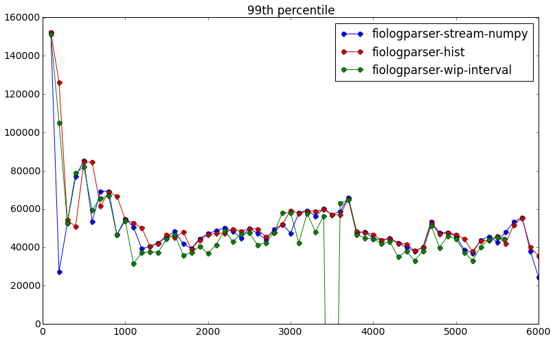
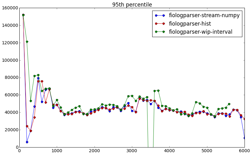
Note that using an end-time of “halfway between current sample and last sample” was determined empirically - the graphs above in the Accuracy section showed a very distinct x-axis offset between the red and blue graphs by 50 milliseconds when the end times were used as-reported by fio. Intuitively this makes sense because the histograms are filled in the e.g. 100 milliseconds before it gets reported. So on average we would expect half the samples to actually complete in the first 50 ms and the other half to actually complete in the second 50 ms. This of course assumes no sinusoidal / clearly periodic pattern of requests of certain latency values, e.g. all high latency requests happening to complete every 100 ms.

Second time issue: We SSH into multiple hosts and run fio in parallel. Let’s say at time t=0 we execute pdsh in CBT on the controller node, with two hosts being started. At times [250,50] fio is started on the two ceph client nodes. The way fio reports interval data is by calculating the time since fio started on the host it is running. Thus if we use the example from the four histogram samples example from the first issue above, we get the same end times of [50.0,55.5,...] when we in fact should be synchronizing the end times to get [100.0, 200.0, 300.5, 305.5, ...] where we have incremented the sample end-times reported by a host by the delay with which it takes for pdsh to start fio.^[e]

Need to verify how fio treats samples with latency larger than the last bin.

Latency Visualization

Possible tools:

Elasticsearch (ES) for data storage
Kibana
D3
Pbench
Processing

Kibana with ES method:

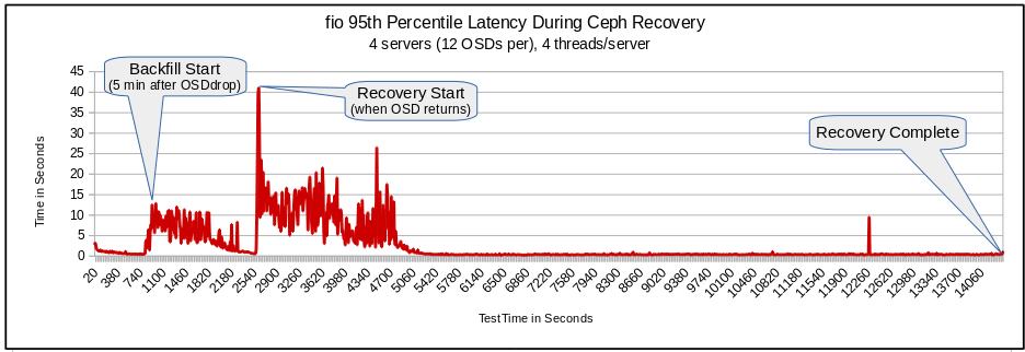
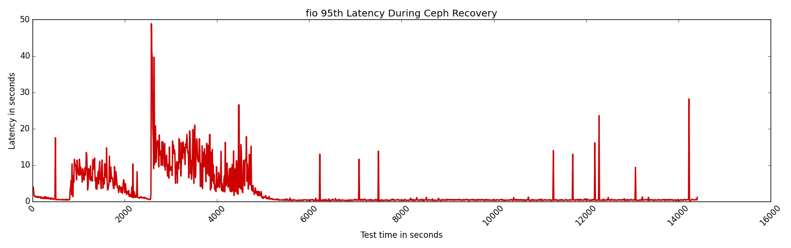
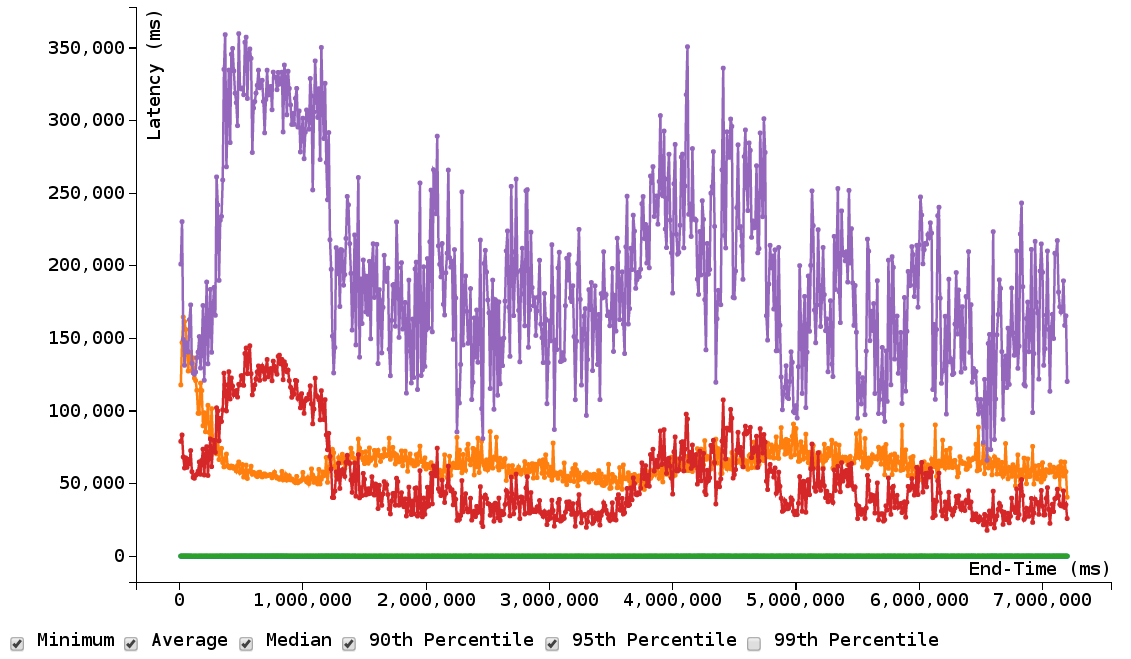
75th, 90th, and 95th percentile plots calculated in ES and plotted in Kibana shown below:

Ease of implementation: Indexing API for ES very straightforward. Scalability: ES clearly designed to scale in terms of amount of data stored. Kibana features allow for auto-refresh viewing last N minutes of data, minimizing data aggregation overhead as samples come in.Portability: Web-browser. Can run ES and Kibana instances anywhere, regardless of viewing location. Usability: Involves running ES and Kibana instances, with graphical frontend to creating new plots. Extensibility: Kibana has interfaces for all the basic statistical aggregation methods given by ES. Not immediately apparent how we would show percentiles in Kibana from histograms stored in ES. Verdict: Probably need more visual implementation flexibility than Kibana allows. Kibana feels tailored more towards e.g. apache log files and other such system logs. It is however sufficient in giving live percentile plots at scale, which is a good baseline for comparing to other visualization methods we try.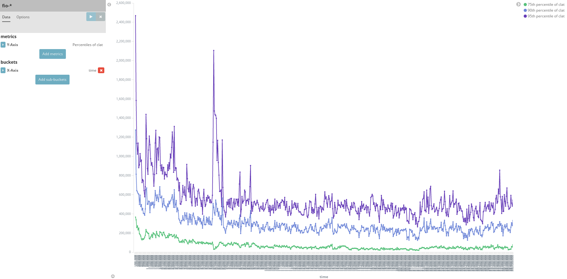

D3 method:

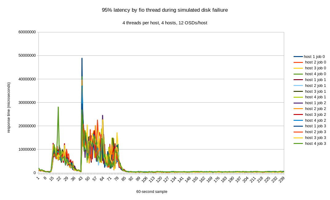
Prototype of plotting percentiles over time in d3:

Ease of implementation: Lots of built-in plotting libraries and tools. Easy to use / don’t need to reinvent existing plotting techniques. Scalability: Can deal with scalability on the data processing side - sampling of histograms and line plots need only be as accurate as the screen can show. Portability: Again, browser-based so can serve and view from anywhere. Usability: Static html and js files on a webserver. Eventually integrate directly into CBT, so even easier to use. Extensibility: Can rely on the plethora of d3 and other javascript libraries to extend the visualizations. Verdict: Should use this method, but look into using pbench and other existing javascript files / libraries / functions.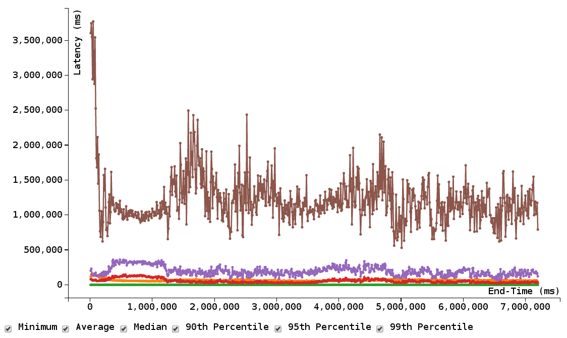

JSChart

Revision history (2016):

June 27, - get ready for review with Mark
July 17

histogram merging & weighting algorithm
How to use fio and fiologparser with histogram output

July 22 - histogram method accuracy in fio histograms section
Aug 3 - JSChart content

[a] I thought this would be handled by measuring interval boundaries in threads based on start_time + interval_num * interval_duration

[b] Are you talking about the drifting problem? I'm referring to the one-time delay caused by SSHing into the hosts and not necessarily starting fio at the same time.

[c] didn't you say you had fixed the code so it handled the fact that fio threads didn't all start at exactly the same time? If so this comment isn't correct anymore, right?

[d] There are two layers to it, one of which I did fix and the second of which may be unimportant (see nested bullets I'm about to add)

[e] This needs to be automated / done in CBT.

Cloud latency measurement problem